| < Previous page | Next page > |
|
Profile Example 1
In this tutorial you will learn how to
You should start CDS, then pick ex5.cdsdat from the Recent Job List, or use File - Open to open “ex5.cdsdat” in the “documents\cds3” folder. When the job opens you will be given the plan view. As CDS does not have an alignment for the center line the values for the Eastings and Northings of each of the points; are set to the Chainage, Offset values of the respective points.
You should pull down the Road menu, and then select the Natural Criteria option that will present a further list of options available.
Select the Profile Parameters option.
Note, as an alternative, you could have selected the Icon marked with an “P” on the icon bar. This “P” refers to the “Profile” lines, and is simply defined as a line joining points with the same attribute on the natural surface. Either way you select it, the screen shown at right will appear.
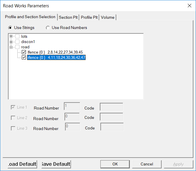
Make sure that you tell the program to "use strings". Next select the "lfence" and the "rfence" string found in the road folder.At this stage you should pull down the Road menu and select the Display & Plotting option followed by Display Profile, and you should get a screen which appears similar to that below. CDS finds the respective strings and creates the profiles based on the chainage and height of the points making up the string.
Providing your display appears similar to that shown, you can now proceed to prepare for plotting.
Setting Plot Parameters
There are two separate sections for creating the parameters that are used in the profile plot. The colour, linetype etc used for each individual profile is in one section. The general parameters that control the scale etc are in another.
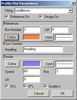
To set the colour and line type make sure that the profile view is visible. Right click within it and a floating menu will appear. You will see the "Plot Parameters" menu at the bottom. Click on it. The dialog as seen above left will appear. As we have two profiles there are two entries in the string at the top. This name is made up of the folder and string ID. Here we have two entries "roadlfence" and "roadrfence". We need to select them in turn.
In this example we have no design lines so the "Design On" tick box can be unticked.
If you select the “Color” box, a window will pop up to offer you a palette of pen colours to choose from , so choose a colour to suit.
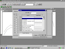
If you select the “Ltype” box, a window displaying available linetypes will appear as seen in the screen above. In this case there is not a great deal of point in using fancy linetypes to plot a simple profile, but you can be creative if you wish, and select something other than a solid or a dashed line.
Normally however, when plotting relatively simple profiles such as these it is usual to use a solid line and use a different colour to differentiate between the distinct profiles.
Note the field named ‘Line Width’ at the top of the screen. This allows you to draw thicker lines by simply increasing the value you set for the line width. Once you have finished playing with the colours and linetypes you should take notice of the field entitled “Box Number”. If you look at the skeleton drawing of a profile below, you will see that each value to be drawn needs to be assigned a “box number” to write the values in.
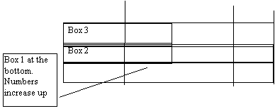
While there are many different formats in use within the Surveying/Engineering Profession, it is quite common to put the value for chainage at the bottom of the profile ie in Box 1, and then organise the other values above it, and that is what we will attempt to do here.
We will place Chainage in Box 1, the values of the Left Fence in Box 2 and those for the Right Fence in Box 3.
Since we are currently defining the left fence and it is already shown in Box 2 no intervention is required.
Select the rfence option from the combo box at the top.
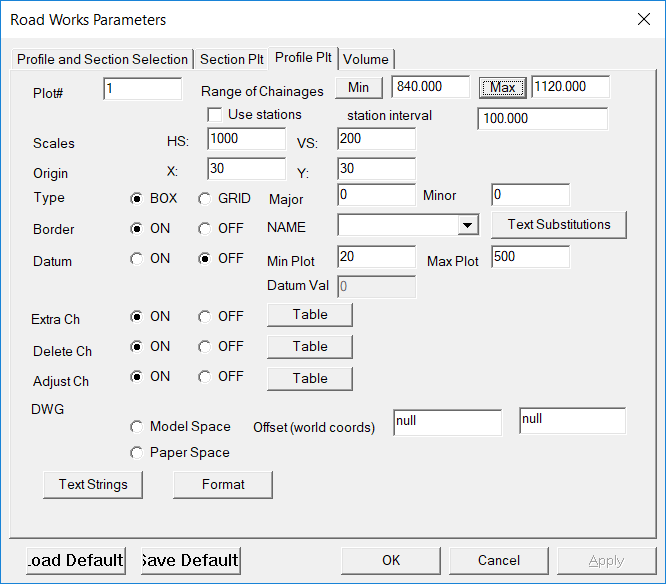
You should enter a Box Number of 3 for this line as it is the right fence, and then OK.
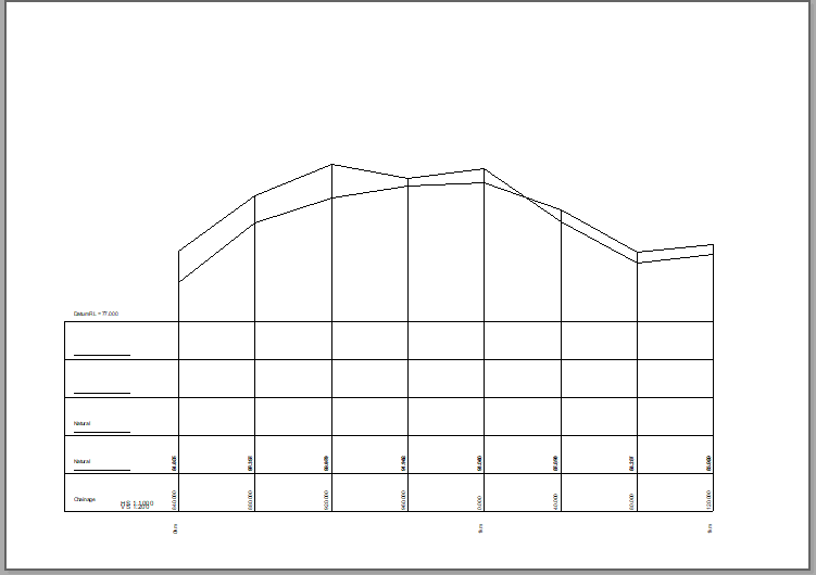
You will however need to alter some of the labels to be placed in the boxes, so select the Format box. You should fill in the screen to the values that appear above, and then select OK to close the parameter screens. Now you are ready for a plot, but you may need to use Print Setup to make sure that you have your plotter selected with A3 paper. Once that is done, you can obtain a Print Preview, which should appear as shown on the next page, and if it does, you may care to plot it out on the plotter.
 |